Transmitter and Waveform#

radarsimpy.Transmitter describes everything that leaves the radar: the shape of the waveform in time and frequency, how many times it repeats and how it is spaced, how each pulse and each channel is modulated, and the geometry and pattern of the transmit array.

This page walks through those four groups in the order they interact. For how the transmitter fits into the rest of the simulation, see Radar System Model.

The Waveform: `f` and `t`#

A transmitter’s waveform is a frequency-versus-time curve, given as a pair of matched arrays. f accepts three forms, and each produces a different kind of radar:

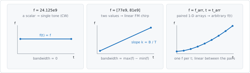
A scalar f gives a tone, a two-element f gives a chirp, matched arrays give an arbitrary sweep — `f` and `t` are always paired sample for sample; the frequency moves linearly between consecutive pairs.#

Form	Result
`f=24.125e9, t=1e-6`	Single-tone CW. A scalar `f` is expanded to `[f, f]` and a scalar `t` to `[0, t]`, so the frequency is flat and `bandwidth` is 0.
`f=[77e9, 81e9], t=[0, 40e-6]`	Linear FM chirp — the FMCW case. The slope is `(f[1] - f[0]) / pulse_length`, available as `radar.chirp_slope`.
`f=f_arr, t=t_arr`	Arbitrary sweep. Any number of matched points; the frequency is linear between them, so a non-linear sweep is approximated by using enough points.

Two derived quantities follow immediately and are used throughout the rest of the simulator:

bandwidth    = max(f) - min(f)
pulse_length = t[-1] - t[0]

t is normalized so that it starts at zero, so only the differences in t matter. pulse_length is the more important of the two: together with the receiver’s fs it fixes samples_per_pulse, and it is the lower bound on the pulse repetition period.

Note

A descending sweep is written the same way — f=[81e9, 77e9] gives a negative chirp_slope. bandwidth stays positive either way, since it is defined from max(f) and min(f).

from radarsimpy import Transmitter

cw    = Transmitter(f=24.125e9, t=1e-6)
fmcw  = Transmitter(f=[77e9, 81e9], t=[0, 40e-6])

# a non-linear (quadratic) sweep, 64 breakpoints
import numpy as np
t_arr = np.linspace(0, 40e-6, 64)
f_arr = 77e9 + 4e9 * (t_arr / 40e-6) ** 2
nlfm  = Transmitter(f=f_arr, t=t_arr)

The Pulse Train: `pulses` and `prp`#

The waveform above describes one pulse. pulses says how many to transmit and prp says how far apart their start times are:

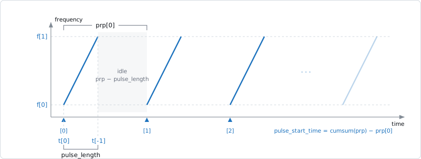
Three chirps spaced by prp, with pulse_length, t and f annotated — `prp` is measured start-to-start, not end-to-start. When it exceeds `pulse_length` the transmitter is idle in between; when it equals `pulse_length` the chirps run back to back, the usual fast-chirp FMCW arrangement.#

The rules the constructor enforces:

prp >= pulse_length for every pulse — the next pulse cannot start before the current one ends.
prp may be a scalar (applied to all pulses) or an array of length pulses.
If prp is omitted it defaults to pulse_length, i.e. 100 % duty cycle.

Pulse start times are the cumulative sum, referenced to the first pulse:

pulse_start_time = cumsum(prp) - prp[0]

which is why a scalar prp gives a uniform train and an array prp gives a staggered one. Staggered PRPs are the standard way to break Doppler ambiguity in pulsed radars:

import numpy as np
from radarsimpy import Transmitter

# alternating 50 us / 60 us PRP over 128 pulses
prp = np.tile([50e-6, 60e-6], 64)
tx = Transmitter(f=[77e9, 81e9], t=[0, 40e-6], pulses=128, prp=prp)

Important

The receive window is one pulse_length long and opens gate_delay after each pulse starts. It does not extend into the idle time between pulses. For a pulsed radar that listens after transmitting rather than during, set the receiver’s gate_delay to move the window onto the range interval you care about — see Long-Range Stretch Processing.

Frequency Hopping: `f_offset`#

f_offset adds a constant frequency shift to each pulse. It is a transmitter-level property, so it applies to all channels alike, and its length must match pulses:

import numpy as np
from radarsimpy import Transmitter

# 64 pulses, hopping in 10 MHz steps
tx = Transmitter(
    f=[24.0e9, 24.1e9],
    t=[0, 20e-6],
    pulses=64,
    prp=25e-6,
    f_offset=np.arange(64) * 10e6,
)

A scalar is broadcast to every pulse. Frequency hopping widens the effective bandwidth across a frame — useful for interference mitigation and for synthetic-bandwidth range processing — but it makes the pulses non-identical, which matters for coherent Doppler processing and for long range gates.

Modulation: Slow Time and Fast Time#

Two independent modulation mechanisms sit on each transmit channel, and the distinction between them is the one worth getting right:

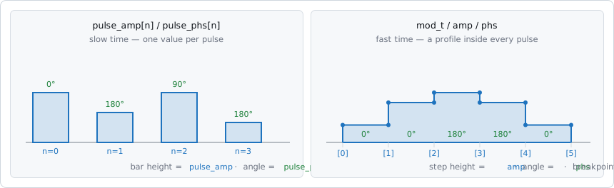
Left: pulse modulation — one amplitude and one phase per pulse, constant across the pulse. Right: waveform modulation — a sampled profile applied inside every pulse, identically from pulse to pulse.#

	Pulse modulation	Waveform modulation
Keys	`pulse_amp`, `pulse_phs`	`mod_t`, `amp`, `phs`
Domain	Slow time (pulse to pulse)	Fast time (within a pulse)
Length	Must equal `pulses`	Any length; `amp`, `phs` and `mod_t` must match each other
Typical use	Phase codes, Doppler-division MIMO, amplitude tapering across a frame	Pulse shaping, intra-pulse phase codes, per-channel frequency offsets

Both are complex gains, combined as amp * exp(1j * phs * pi / 180), and both default to unity.

Pulse modulation#

pulse_amp and pulse_phs are per-channel sequences of length pulses. The classic use is separating MIMO transmit channels by code:

import numpy as np
from radarsimpy import Transmitter

pulses = 128

# Doppler-division MIMO: each Tx gets its own phase ramp across the frame,
# which shifts its returns to a different Doppler bin.
n = np.arange(pulses)
channels = [
    {"location": (0, 0, 0),        "pulse_phs": np.zeros(pulses)},
    {"location": (0, 0.006, 0),    "pulse_phs": (180 * n) % 360},
]

tx = Transmitter(
    f=[77e9, 81e9], t=[0, 40e-6], pulses=pulses, prp=50e-6, channels=channels
)

Waveform modulation#

mod_t carries the timestamps and amp / phs the profile applied at those instants. The profile is sampled with a zero-order hold — the value in force at a given instant is the one from the nearest preceding breakpoint, not an interpolation — and it repeats identically in every pulse.

Together these three are an arbitrary complex envelope, which is what makes waveforms outside the FM family reachable: a phase code, a shaped pulse, or an OFDM symbol obtained by loading subcarriers and taking an IFFT all reduce to amp and phs sampled on the mod_t grid. Because the table repeats per pulse, one symbol is direct while a frame carrying different data in each symbol takes more than one call — see Radar System Model.

Important

mod_t must be equally spaced and increasing. The simulator derives the step from mod_t[1] - mod_t[0] and indexes the table arithmetically, so unevenly spaced timestamps are silently misread. Use np.linspace(0, pulse_length, n) and choose n for the time resolution you need.

A raised-cosine transmit taper, for example:

import numpy as np
from radarsimpy import Transmitter

pulse_length = 40e-6
mod_t = np.linspace(0, pulse_length, 256)
taper = 0.5 - 0.5 * np.cos(2 * np.pi * np.arange(256) / 255)

tx = Transmitter(
    f=[77e9, 81e9],
    t=[0, pulse_length],
    pulses=128,
    prp=50e-6,
    channels=[{"location": (0, 0, 0), "mod_t": mod_t, "amp": taper}],
)

Supplying only phs fills amp with ones, and supplying only amp fills phs with zeros, so either can be used alone.

Separating MIMO channels#

A virtual array is only meaningful when the transmit channels can be told apart in the received signal (see Radar System Model). The mechanisms available are:

Scheme	Configured with	Notes
TDM	Per-channel `delay`	Each channel fires at a different offset within the PRP. Simple and fully orthogonal, at the cost of an \(M\)-fold reduction in the effective PRF per channel.
CDM	Per-channel `pulse_phs`	Orthogonal phase codes over the frame, e.g. rows of a Hadamard matrix. All channels transmit at once, so no PRF is lost.
DDM	Per-channel `pulse_phs` ramp	A progressive phase shift moves each channel to its own Doppler band. Costs unambiguous Doppler span rather than PRF.
Intra-pulse	Per-channel `mod_t` / `amp` / `phs`	Phase codes or a linear phase ramp (a frequency offset) applied inside each pulse. The ramp resolution is limited by the `mod_t` step.

Pulsed Waveforms#

A pulsed radar transmits briefly and then listens for a long time, and that does not map onto t the way a chirp does. The rule to internalise:

Important

t is the receive window, not the transmit duration.

For CW and FMCW the two coincide — the transmitter is on for the whole sweep, so one number describes both. For a pulsed radar they differ by orders of magnitude, and the split is expressed with the fast-time amplitude gate:

t spans the entire pulse repetition interval. That is what sets pulse_length, samples_per_pulse and, by default, prp.
amp and mod_t switch the transmitter on for the first \(\tau\) seconds of that interval and off for the rest.

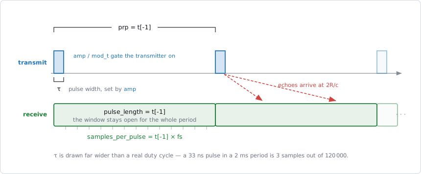
Pulsed radar timing, with t spanning the listening window and amp gating the transmitter — The blue pulse is the transmitter being gated on; the green band is the receive window, which stays open for the whole period. Both are described by the same `t` — the narrow one through `amp`, the wide one directly.#

A rectangular pulse#

import numpy as np
from scipy import constants
from radarsimpy import Radar, Transmitter, Receiver

c = constants.c
fc = 10e9            # carrier
prf = 20e3           # pulse repetition frequency
fs = 20e6            # ADC rate
pulse_width = 0.5e-6 # tau

prp = 1 / prf                          # 50 us listening window
n = int(round(prp * fs))               # samples in that window

mod_t = np.arange(n) / fs
amp = np.zeros(n)
amp[mod_t < pulse_width] = 1.0         # transmitter on for the first tau

tx = Transmitter(
    f=fc,                              # single tone: an unmodulated pulse
    t=prp,                             # the whole interval, not the pulse
    tx_power=40,
    pulses=256,
    channels=[{"location": (0, 0, 0), "mod_t": mod_t, "amp": amp}],
)

rx = Receiver(fs=fs, noise_figure=5, rf_gain=20, baseband_gain=30,
              channels=[{"location": (0, 0, 0)}])

radar = Radar(transmitter=tx, receiver=rx)

prp is not passed: it defaults to pulse_length, which is already the full interval. Passing prp=1/prf explicitly is equivalent.

Quantity	Expression	This example
Samples per pulse	`prp * fs`	1000
Transmit-on samples	`tau * fs`	10
Duty cycle	`tau / prp`	1 %
Max unambiguous range	`c * prp / 2`	7.49 km
Range resolution	`c * tau / 2`	75 m
Range per sample	`c / (2 * fs)`	7.5 m

A target at range \(R\) puts its echo at roughly sample \(2R f_s / c\), spread over the \(\tau f_s\) samples the pulse occupies. A point target at 1500 m in the configuration above lands within one sample of index 200, which back-converts to 1491 m — inside a single 7.5 m range bin.

How far `mod_t` should span#

The snippet above builds mod_t across one interval. Spanning the whole frame instead — np.arange(int(prp * pulses * fs)) / fs — is equally valid, and the choice decides what happens to a target beyond the unambiguous range \(c \cdot \text{prp} / 2\):

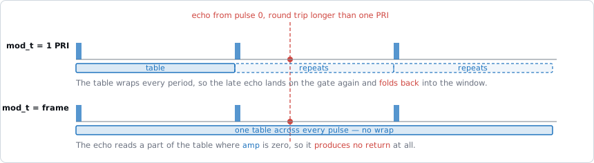
A one-period modulation table wraps and folds late echoes; a frame-long table does not — The modulation table is indexed by time within a pulse, so a one-period table repeats every period while a frame-long table does not. A late echo therefore reads a gated-on sample in the first case and a gated-off sample in the second.#

`mod_t` spans	One interval	The whole frame
Length	`int(prp * fs)`	`int(prp * pulses * fs)`
Target beyond \(R_\text{max}\)	Folds back to \(R - c\,\text{prp}/2\), as real hardware does	Returns exactly zero — never seen
Use when	Range ambiguity is part of what you are studying	You want only unambiguous returns, which is usually simpler

With the 80 µs interval above and a target at 14 km, a one-interval table places the folded echo at samples 79–81, which is 2 km — where a real radar would report it. A frame-long table returns nothing for that target at all.

A chirped pulse#

An unmodulated pulse trades range resolution against energy on target: making \(\tau\) shorter sharpens the range profile but transmits less. Pulse compression breaks that trade by sweeping the frequency within the pulse.

Since f and t are matched arrays, the sweep can be confined to the first \(\tau\) and held flat for the remainder, which is exactly where amp has already switched the transmitter off:

bandwidth = 10e6

tx = Transmitter(
    f=[fc - bandwidth / 2, fc + bandwidth / 2, fc + bandwidth / 2],
    t=[0, pulse_width, prp],
    tx_power=40,
    pulses=256,
    channels=[{"location": (0, 0, 0), "mod_t": mod_t, "amp": amp}],
)

The three points sweep across the pulse and then hold. bandwidth reports 10 MHz and pulse_length is still the full 50 µs interval, so samples_per_pulse is unchanged. Range resolution after matched filtering becomes \(c / 2B\) — 15 m here, against 75 m for the rectangular pulse of the same duration.

Note

The simulator returns the received echo, not a compressed range profile. Matched filtering is a post-processing step you apply to result["baseband"] — correlate each pulse against the transmitted waveform, then continue with Doppler processing as usual.

Practical notes#

Eclipsing. A target close enough that its echo returns while the transmitter is still on falls inside the first \(\tau f_s\) samples. Real hardware is deaf there; the simulator is not, so those samples need discarding by hand if you are modelling a system with a real duplexer.
Duty cycle. Realistic values are small — the SAR example on radarsimx.com gates 3 samples out of 120 000. Long windows at a high fs make samples_per_pulse large, and memory scales with it.
Range gating. For long-range work, opening the window at the interval of interest rather than at zero delay avoids sampling empty space; see Long-Range Stretch Processing.
Staggered PRF. prp accepts an array, so the interval can vary pulse to pulse to break Doppler ambiguity. Because t also sets the window length, and prp >= pulse_length is enforced, the stagger can only extend intervals beyond t[-1], never shorten them: set t to the shortest interval you want and stagger upward from there. Every receive window keeps the same length regardless, so a longer interval simply adds dead time after the window closes.

Transmit Channels#

channels is a list of dictionaries, one per transmit element. location is the only required key.

Key	Default	Meaning
`location`	—	`[x, y, z]` in metres, relative to the radar origin.
`polarization`	`[0, 0, 1]`	Antenna polarization vector. Vertical `[0, 0, 1]`, horizontal `[0, 1, 0]`, right-hand circular `[0, 1, 1j]`, left-hand circular `[0, 1, -1j]`.
`delay`	`0`	Transmit start delay in seconds. This is the TDM knob, and it shifts the channel’s timestamps.
`azimuth_angle` / `azimuth_pattern`	`[-90, 90]` / `[0, 0]`	Matched arrays of angle (degrees) and gain (dB).
`elevation_angle` / `elevation_pattern`	`[-90, 90]` / `[0, 0]`	Same, in elevation.
`grid`	`1`	Angular step in degrees of the grid used to test scene occupancy during ray tracing. Affects mesh simulations only.
`pulse_amp` / `pulse_phs`	`1` / `0`	Slow-time modulation, length `pulses`.
`mod_t` / `amp` / `phs`	`None`	Fast-time modulation.

Antenna patterns and gain#

Patterns are given in dB against angle, and the two cuts are not treated symmetrically:

The peak of the azimuth pattern becomes the channel’s antenna gain (txchannel_prop["antenna_gains"]), and the azimuth pattern is then normalized to that peak.
The elevation pattern is normalized to its own peak and contributes shape only.

So put the absolute gain in azimuth_pattern and use elevation_pattern purely for the elevation cut’s shape. A channel with a 12 dBi peak and a 60° azimuth beamwidth:

channel = {
    "location": (0, 0, 0),
    "azimuth_angle": [-90, -30, 0, 30, 90],
    "azimuth_pattern": [-10, 9, 12, 9, -10],   # peak 12 dB -> antenna gain
    "elevation_angle": [-90, -20, 0, 20, 90],
    "elevation_pattern": [-20, -3, 0, -3, -20],  # shape only
}

Angles follow the conventions in Coordinate Systems.

Power and Phase Noise#

tx_power is the transmit power in dBm and scales the returned signal directly. pn_f and pn_power describe the oscillator’s single-sideband phase-noise profile — frequency offsets in Hz against power in dBc/Hz — and must be supplied together:

tx = Transmitter(
    f=[77e9, 81e9],
    t=[0, 40e-6],
    tx_power=15,
    pulses=128,
    prp=50e-6,
    pn_f=[1e3, 1e4, 1e5, 1e6],
    pn_power=[-80, -90, -100, -110],
)

Because the receiver deramps against the same oscillator, phase noise partially cancels for short delays and is progressively less correlated at longer ones. Noise Simulation covers the model and this range dependence in detail.

Reading the Configuration Back#

tx.bandwidth           # max(f) - min(f), Hz
tx.pulse_length        # t[-1] - t[0], s
tx.num_pulses
tx.num_channels
tx.channel_locations   # [M, 3]
tx.get_channel_info(0) # location, polarization, delay, gain, patterns

tx.waveform_prop["pulse_start_time"]
tx.txchannel_prop["antenna_gains"]

Transmitter and Waveform#

The Waveform: f and t#

The Pulse Train: pulses and prp#

Frequency Hopping: f_offset#

Modulation: Slow Time and Fast Time#

Pulse modulation#

Waveform modulation#

Separating MIMO channels#

Pulsed Waveforms#

A rectangular pulse#

How far mod_t should span#

A chirped pulse#

Practical notes#

Transmit Channels#

Antenna patterns and gain#

Power and Phase Noise#

Reading the Configuration Back#

See Also#

The Waveform: `f` and `t`#

The Pulse Train: `pulses` and `prp`#

Frequency Hopping: `f_offset`#

How far `mod_t` should span#