Ray-Tracing Simulation

This page describes the parameters of sim_radar that control the ray-tracing and Physical Optics (PO) based simulation for 3D mesh targets, as well as the target-level flags that affect how individual objects are handled during the simulation.

sim_radar Parameters

The following parameters of sim_radar control the mesh simulation behavior:

density

Type:

float

Default:

1.0

Ray density, defined as the number of rays per wavelength. This parameter directly controls how many rays are launched towards each occupied grid cell during the pyramid ray generation stage.

• Higher values produce more rays, leading to finer spatial sampling of the target surface and more accurate PO results, at the cost of increased computation time and GPU/CPU memory usage.

• Lower values reduce the number of rays for faster computation, but may miss small geometric features or produce less accurate scattering results.

A value of 1.0 means one ray per wavelength, which is generally a reasonable starting point. Increase the density for scenes requiring higher fidelity, or decrease it below 1.0 for faster computation when high spatial resolution is not needed or when the target mesh faces are large relative to the wavelength.

Tip

Individual targets can override the global density by setting a per-target density value in the target dictionary. When a target’s density is 0.0 (the default), the global density from sim_radar is used.

level

Type:

str or None

Default:

None

Sets the simulation fidelity: how often the scene geometry is re-traced as the radar works its way through a frame.

• None or "frame" — one ray-tracing pass per frame

• "pulse" — one pass per pulse

• "sample" — one pass per ADC sample

How often the scene is re-traced

A radar frame is a grid of pulses and samples, and the level decides how that grid is carved up into ray-tracing passes:

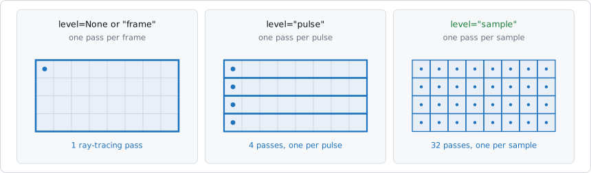
Each grid is one radar frame of a single transmit channel: rows are pulses, columns are ADC samples. A blue region is what one pass covers.

For a frame of P pulses of S samples, each transmit channel costs one pass at "frame", P passes at "pulse", and P × S passes at "sample". A 128-pulse, 256-sample frame is therefore 1 pass, 128 passes, or 32768 passes — and the run time follows that count closely.

What happens between passes

Within a pass the scene is not simply frozen. Each target is carried forward from the traced instant at its range rate — a straight line at constant speed. That is exact for a target translating at constant velocity, and progressively wrong for anything else:

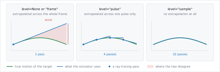
Horizontal axis: time within one frame; vertical axis: range to a point on the target. Teal is the true motion, blue is what the simulator uses, red is where they disagree. Each pass restarts from the true geometry, so the blue track steps back onto the curve at every one.

Rotation, vibration, angular acceleration and any curved path are what the straight line misses. The further a pass has to reach, the larger the discrepancy — so the level you need is set by how much the scene changes during one frame, not by how fast the targets are moving in absolute terms.

Choosing a level

• None or "frame" — static scenes, and any motion that is linear or close enough to it across one frame. That covers more ground than it sounds: when the pulse repetition rate is high compared with the rate at which the target’s motion changes, a whole frame spans only a small slice of that motion, and the straight line holds well. The fastest option, and the right starting point.

• "pulse" — motion that curves appreciably over a frame but not within a single pulse. A good balance when the frame is long enough, or the dynamics fast enough, that one straight line no longer covers it.

• "sample" — rotating, vibrating or accelerating targets. Required for micro-Doppler work: the modulation you are trying to see lives inside a pulse, which is exactly what the lower levels smooth away.

Note

Because cost tracks the number of passes, "sample" can be orders of magnitude slower than "frame" on the same scene. When a micro-Doppler study genuinely needs it, it is usually worth trimming the frame down to the pulses you actually intend to process.

ray_filter

Type:

list or None

Default:

None

Filters rays based on their number of reflections (bounces). When set, only rays whose reflection count falls within the range [ray_filter[0], ray_filter[1]] are included in the baseband calculation.

• ray_filter[0] — Minimum number of reflections (inclusive).

• ray_filter[1] — Maximum number of reflections (inclusive).

When None, no filtering is applied and all rays from the minimum default to the maximum allowed reflections are included.

This is useful for isolating specific scattering mechanisms. For example:

• ray_filter=[1, 1] — Include only single-bounce (direct) reflections.

• ray_filter=[2, 3] — Include only double- and triple-bounce reflections.

The count is the path’s own, end to end. With back_propagating enabled a return may reflect on its way out as well as on its way in, and those reflections count too — a path that reaches a target over three bounces and leaves over one more is four, not three.

ray_filter[1] also caps how deep rays are traced, since a bounce past it could not contribute anyway. That makes it a little more than a filter: a ray stopped by the cap is treated as still travelling, so it contributes no outgoing reflections (see back_propagating below).

back_propagating

Type:

bool

Default:

False

Lets a scattering point send energy back to the receiver by reflecting off the surfaces the ray arrived over, rather than only in a straight line.

Rays are traced away from the radar, and a scattering point normally radiates straight back to the receiver. That misses the returns that leave a target, bounce off something, and only then arrive — the paths that matter inside a tunnel, where energy reaches the radar off the walls, ceiling and floor rather than directly.

With this enabled, a ray that leaves the scene also contributes returns that reflect their way back out over the surfaces it came in over. Each one is checked before it counts: the reflection has to land on the surface rather than past its edge, and nothing may stand in the way. Chains are only built for a ray that genuinely escaped, never one the trace depth stopped — that ray may well have carried on in reality, and the bounce it would have taken next is the ordinary forward path’s to describe.

Note

Enabling back propagation costs more scattering evaluations per snapshot, which are the dominant cost of a mesh simulation. It adds nothing at all to a scene where rays do not bounce: a single convex target returns exactly the same baseband either way.

Target Flags

The following flags can be set in the target dictionary for 3D mesh targets to modify how the simulator handles them.

skip_diffusion

Type:

bool

Default:

False

Marks a surface as a pure reflector. It goes on redirecting rays exactly as before, but it no longer contributes a scattered return of its own.

This is meant for large flat reflectors — ground planes, building walls, the inside of a tunnel — where the surface reflects specularly, away from the radar, so its own backscatter is negligible next to the targets in the scene.

Effect on the returned signal

A ray sends energy back to the receiver only once it has touched a surface that is not skipped. Bounces on skipped surfaces before that point redirect the ray and do nothing else:

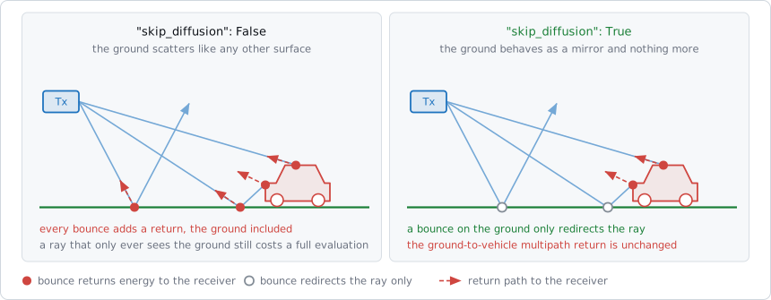
A filled marker is a bounce that returns energy to the receiver; a hollow one only redirects the ray onwards.

So a ray that leaves the radar, strikes the ground and carries on out of the scene contributes nothing at all, while radar → ground → vehicle → radar is captured in full, along with every bounce after the vehicle. The multipath structure of the scene survives intact; what disappears is the direct return of the flat surface itself.

Effect on cost

In a scene framed by a ground plane, a large share of the rays land on the ground and nowhere else. skip_diffusion removes that work twice over: directions that see nothing but a skipped surface are dropped before any rays are launched into them, and the bounces that do happen on it add no scattering evaluation against the receive channels. Those evaluations are the dominant cost of a mesh simulation, so this is usually the largest single saving available on a ground-plane scene — and a much larger one than environment offers.

When to use it

Set skip_diffusion=True for:

• ground planes and terrain surfaces

• building walls, tunnel linings and large barriers

• any surface flat and large enough that its own backscatter does not matter

Leave it at False for:

• the targets whose returns you are measuring

• curved or faceted surfaces, which do scatter back towards the radar

• small surfaces, where “large and flat” does not really hold

environment

Type:

bool

Default:

False

Marks a target as part of the surroundings rather than as something you are measuring. Ground planes, terrain, building walls and tunnel linings are environment objects; the vehicle, pedestrian or corner reflector under test is not.

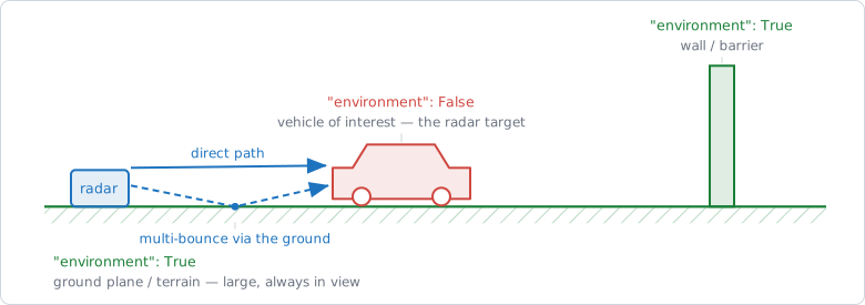
The surroundings carry the flag, the vehicle under test does not. Both still scatter, and the ground-bounce path is simulated either way.

An environment object still takes part in the simulation in exactly the same way as any other target. It reflects according to its permittivity, it contributes its own return, and multi-bounce paths that run through it — radar to ground to vehicle and back — are traced as usual. The flag does not change the physics of a reflection. It changes how many rays are spent on it.

Effect on ray density

Rays are a finite budget, and the simulator spreads that budget across the surfaces it can see. Surrounding surfaces are almost always the largest meshes in a scene and fill most of the field of view, so without the flag they absorb the bulk of the rays — and the target you actually care about is left with whatever remains.

Setting environment=True shifts part of that budget away from the surface and onto the primary targets:

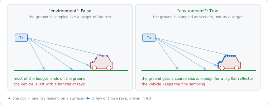
One dot is one ray landing on a surface. Only four of those rays are drawn in full, to keep the fan readable.

The saving is real but modest. It comes from the surface no longer claiming directions its geometry does not actually cover, and from a target behind it setting the sampling rather than the surface itself. Rays that land on the surface and nowhere else are still launched, and still evaluated.

Note

If what you want is those rays gone, skip_diffusion is the flag that does it, and it saves considerably more than environment does. Reach for environment when the surface still has to scatter properly.

Effect on the PO calculation

Every ray that lands on a surface contributes one surface-current sample to the Physical Optics integral, so ray density is really surface sampling density. A coarser share of the budget means larger facets on the environment surface:

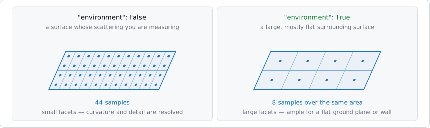
The same patch of surface at two sampling densities. Each dot is one ray landing, and so one surface-current sample in the PO integral.

Those samples still use the permittivity you set and still feed the same PO integral. What coarser sampling costs is surface detail. A large flat ground plane or wall scatters much the same whether it is sampled finely or coarsely, which is precisely why the flag is safe there. A small, curved or intricate surface does not, so it should keep the full density.

When to use it

Set environment=True for:

• terrain, embankments and other large surroundings that still scatter usefully back towards the radar

• any large surface that frames the scene rather than being measured in it, and whose own return you want to keep

Leave it at False for:

• the vehicles, pedestrians or reflectors whose returns you are measuring

• small or strongly curved objects, where surface detail drives the result

• any surface whose own RCS is the quantity of interest

• anything already marked skip_diffusion=True — that flag covers the same sampling treatment, so environment adds nothing. See Choosing between the two flags below.

Choosing between the two flags

The two flags are easy to confuse because they are recommended for the same kinds of object. They do act on different things:

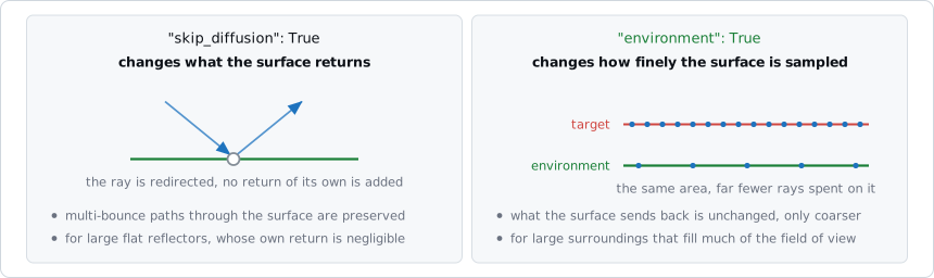
Left: the bounce is drawn hollow because the surface adds no return of its own. Right: one surface sampled densely as a target, sparsely as environment.

• skip_diffusion decides what the surface sends back. Set it when the surface is flat enough that its own return is not worth computing.

• environment decides how finely the surface is sampled. Set it when the surface is large enough that sampling it at full density would starve the real targets of rays.

Important

skip_diffusion=True already covers what environment does to sampling. Setting both on the same surface gains nothing, and can cost extra rays — pick one.

So in practice:

• Large flat reflector whose own return does not matter — a ground plane, a wall, a tunnel lining. skip_diffusion=True on its own is enough:

  ground = {
      "model": "./models/ground.stl",
      "location": (0, 0, 0),
      "skip_diffusion": True,
  }
  

• Large surrounding surface whose return you do want, but which is too big to be sampled like a target — a broad embankment, a terrain mesh you are bouncing signals off. environment=True on its own is the flag for this, and it is the only case where environment does real work:

  terrain = {
      "model": "./models/terrain.stl",
      "location": (0, 0, 0),
      "environment": True,
  }
  

• A target you are measuring — neither flag.

See Also

• Animated Targets (glTF 2.0 / GLB) - Driving mesh targets from keyframed glTF motion

• Coordinate Systems - Placing and orienting targets in the scene

• Usage Examples - Ray-tracing and RCS examples