Noise Simulation

RadarSimPy models two distinct noise sources that affect radar signal quality: receiver thermal noise, introduced at the receiver front-end, and transmitter phase noise, arising from oscillator imperfections in the transmitter. Both are described in the sections below.

Receiver Thermal Noise

RadarSimPy simulates thermal noise at the receiver. This section describes the statistical properties of the generated noise and how it behaves in single-channel and MIMO radar configurations.

Noise Properties

The receiver noise has the following properties:

• Gaussian white noise — zero-mean, with standard deviation determined by the receiver noise parameters (noise figure, gains, bandwidth, and load resistance).

• Independent across frames — each frame receives a fresh, independent noise realization.

• Independent across Rx channels — different physical Rx channels have statistically independent noise.

• Deterministic given a seed — when a random seed is provided, the noise is fully reproducible.

Complex vs. Real Baseband

• Complex baseband (bb_type="complex"): noise has both real and imaginary components. Each component is an independent Gaussian with standard deviation \(\sigma / \sqrt{2}\), so the total RMS amplitude equals \(\sigma\).

• Real baseband (bb_type="real"): noise is purely real with standard deviation \(\sigma\).

Same Timestamp, Same Rx → Same Noise

A key property of the noise simulation is:

Important

If two output samples belong to the same physical Rx channel and correspond to the same timestamp, they receive exactly identical noise values — regardless of how many virtual channels share that combination.

The noise value for each sample is a deterministic function of three identifiers:

1. Frame index — which frame the sample belongs to.

2. Physical Rx channel — determined by rx_ch = ch_idx % rx_size.

3. Absolute sample index — the sample’s position on the discrete time grid (timestamp offset from the minimum, quantized by the sampling rate).

Because the function is deterministic, any two samples with the same (frame_idx, rx_ch, absolute_sample_index) tuple always produce the same noise value. No lookup table or shared buffer is required.

Noise in MIMO Configurations

In a MIMO radar with \(M\) Tx and \(N\) Rx channels, the simulator produces \(M \times N\) virtual channels per frame. The virtual channels are ordered as:

ch[0]         = Tx0 → Rx0
ch[1]         = Tx0 → Rx1
...
ch[N-1]       = Tx0 → Rx(N-1)
ch[N]         = Tx1 → Rx0
ch[N+1]       = Tx1 → Rx1
...
ch[M*N - 1]   = Tx(M-1) → Rx(N-1)

Each virtual channel maps to a physical Rx channel via:

\[\text{rx\_ch} = \text{ch\_idx} \mod N\]

Virtual Channel Grouping

All virtual channels that share the same physical Rx and have the same transmit timing (i.e., identical timestamps) will contain identical noise. For example, with 2 Tx and 2 Rx:

ch[0] = Tx0 → Rx0    ─┐
ch[2] = Tx1 → Rx0    ─┘  Same Rx0, same timing → identical noise

ch[1] = Tx0 → Rx1    ─┐
ch[3] = Tx1 → Rx1    ─┘  Same Rx1, same timing → identical noise

This matches the physical reality: the noise originates at the receiver front-end, so all signal paths through the same Rx channel at the same time experience the same thermal noise.

Note

If the Tx channels have different timing offsets (e.g., TDM-MIMO with staggered pulse timing), each Tx fires at a different time. In that case, even though two virtual channels share the same Rx, they sample the noise at different time indices and thus receive different noise values.

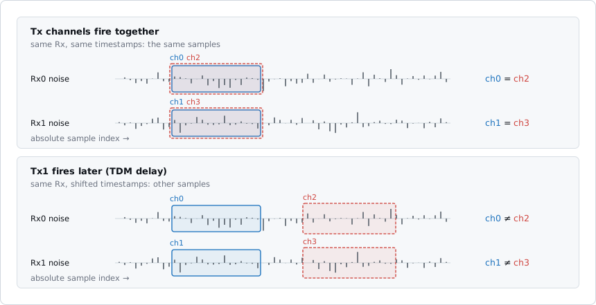
Each physical Rx has one noise stream per frame, laid out on the absolute sample grid. A virtual channel reads the stretch of its Rx stream that its own timestamps select. Top: both Tx channels fire together, so ch0 and ch2 read the same Rx0 samples. Bottom: a Tx1 delay moves ch2 and ch3 to later samples, which are independent.

Impact on MIMO Signal Processing

When performing MIMO beamforming or angle estimation:

• Noise correlation: virtual channels sharing the same Rx have fully correlated noise. The noise covariance matrix across virtual channels is not a scaled identity — it has block structure reflecting the Rx grouping.

• Effective independent noise sources: only \(N\) independent noise realizations exist (one per physical Rx), duplicated across the \(M\) Tx paths that share the same timing.

• SNR estimation: the noise power per virtual channel equals the physical Rx noise power. Averaging across virtual channels that share the same Rx does not reduce noise because the samples are identical.

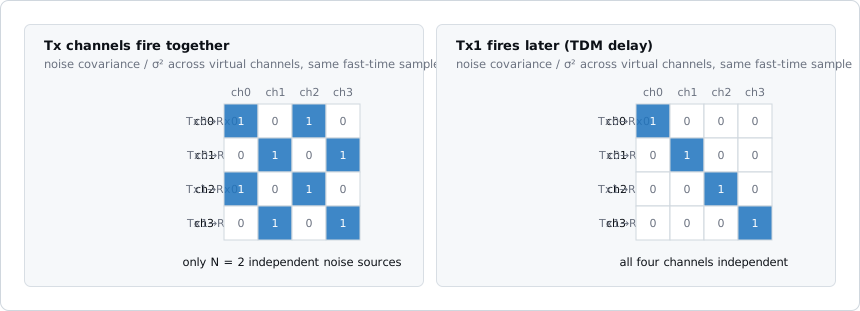
The noise covariance of the 2 Tx × 2 Rx example, taken at the same fast-time sample. When both Tx channels fire together, ch0/ch2 and ch1/ch3 are fully correlated, giving the block structure. A Tx delay puts them on different sample indices, and the matrix becomes the identity.

Example

import numpy as np
from radarsimpy import Radar, Transmitter, Receiver
from radarsimpy.simulator import sim_radar

# 2 Tx, 2 Rx MIMO radar
tx = Transmitter(
    f=[24.075e9, 24.175e9],
    t=80e-6,
    tx_power=10,
    prp=100e-6,
    pulses=4,
    channels=[{"location": (0, 0, 0)}, {"location": (0, 0, 0)}],
)
rx = Receiver(
    fs=2e6,
    noise_figure=10,
    rf_gain=20,
    load_resistor=500,
    baseband_gain=30,
    bb_type="complex",
    channels=[{"location": (0, 0, 0)}, {"location": (0, 0, 0)}],
)
radar = Radar(transmitter=tx, receiver=rx)

result = sim_radar(radar, targets=[{"location": (200, 0, 0), "rcs": 10}])
noise = result["noise"]

# Virtual channels: ch0=Tx0-Rx0, ch1=Tx0-Rx1, ch2=Tx1-Rx0, ch3=Tx1-Rx1
# ch0 and ch2 share Rx0 with same timing → identical noise
assert np.array_equal(noise[0], noise[2])

# ch1 and ch3 share Rx1 with same timing → identical noise
assert np.array_equal(noise[1], noise[3])

# Different Rx channels have independent noise
assert not np.array_equal(noise[0], noise[1])

Multi-Frame Behavior

When simulating multiple frames, each frame generates an independent noise realization. Virtual channels in different frames always have different noise, even if they share the same physical Rx channel:

# With 2 frames, 1 Tx, 1 Rx:
# ch[0] = Frame 0, ch[1] = Frame 1
assert not np.array_equal(noise[0], noise[1])

This ensures that frame-to-frame processing (e.g., Doppler estimation) sees independent noise across slow-time snapshots.

Transmitter Phase Noise

RadarSimPy models transmitter oscillator phase noise using a VCO-based SSB (single-sideband) phase noise model. Phase noise is configured on the Transmitter via the pn_f and pn_power parameters.

Model Overview

If the oscillator output is:

\[V(t) = V_0 \cos\bigl(\omega_0 t + \phi(t)\bigr)\]

then \(\phi(t)\) is the phase noise process. Under the narrowband approximation (valid for any usable system):

\[V(t) \approx V_0 \bigl[\cos(\omega_0 t) - \sin(\omega_0 t)\,\phi(t)\bigr]\]

which is equivalent to multiplying the complex baseband signal by \(e^{-j\phi(t)}\). In other words, \(e^{jx} \approx 1 + jx\) for small \(x\).

Parameters

Phase noise is specified as a SSB power spectral density profile:

• pn_f — frequency offsets from the carrier (Hz), non-negative, 1-D array.

• pn_power — SSB phase noise power at each offset (dBc/Hz), 1-D array of the same length as pn_f.

The profile is interpolated onto the baseband frequency grid \([0,\, f_s/2]\), linearly in log-frequency between points. A 0 dBc/Hz point is added at DC, but on a log-frequency axis DC lies arbitrarily far to the left. Below the first pn_f the level therefore stays at the first pn_power, and the DC bin itself is removed. Above the last pn_f the last pn_power holds up to \(f_s/2\).

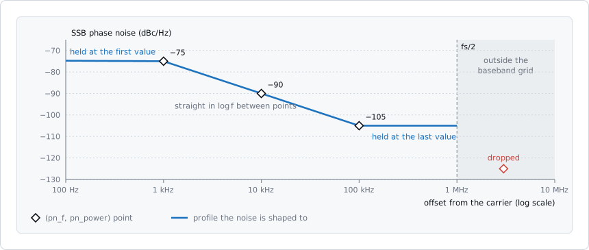
pn_f = [1e3, 1e4, 1e5, 3e6], pn_power = [-75, -90, -105, -125] with fs = 2e6. The three points below \(f_s/2\) are joined by straight lines in log-frequency and held flat at either end. The 3 MHz point lies above \(f_s/2\), so it is dropped.

Phase Noise Properties

Shared synthesizer across all Tx channels

Phase noise is modelled at the transmitter level, not per channel. All Tx channels in an antenna array share a single synthesizer, so they experience exactly the same phase noise process \(\phi(t)\). A single phase noise realization is generated once per frame and applied identically to every Tx channel.

Independent across frames

Each frame receives a fresh, statistically independent phase noise realization. When a deterministic seed is supplied the per-frame seed is derived as \(\text{seed} + \text{frame\_idx}\), guaranteeing reproducibility while keeping frames uncorrelated.

Deterministic given a seed

Providing the same seed to Radar always produces the same phase noise sequence for every frame, enabling reproducible simulations and unit tests.

Impact on Radar Return Signals

Phase noise modulates the transmitted waveform and therefore appears on every received echo. Its effect on the baseband (IF) signal depends on the two-way propagation delay \(\tau\) of the target:

\[s_{\mathrm{IF}}(t) \propto e^{\,j[\phi(t) - \phi(t-\tau)]}\]

• Range correlation effect — because the same oscillator drives both the transmitter and the receiver LO mixer, the transmitted phase noise \(\phi(t)\) and the delayed replica \(\phi(t-\tau)\) are correlated. For short-range targets (\(\tau \ll 1/f_{\mathrm{3dB}}\), where \(f_{\mathrm{3dB}}\) is the corner frequency of the phase noise spectrum) the two terms nearly cancel and the residual IF phase noise is small.

• Long-range degradation — as \(\tau\) increases the correlation decreases and the residual phase noise grows, raising the noise floor and degrading the signal-to-noise ratio for distant targets.

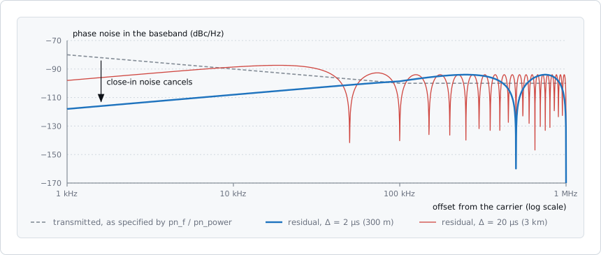
The residual phase noise is the transmitted profile scaled by \(4\sin^2(\pi f \Delta)\). Here \(\Delta\) is the delay between the echo and the reference: the round trip \(\tau\), or \(\tau\) minus gate_delay when a range gate is set. The profile is the one from the example below. At 1 kHz offset the close-in noise is suppressed by about 40 dB at 300 m, but only about 20 dB at 3 km. The longer delay also stops cancelling at a lower offset, above which the response becomes a comb of nulls spaced \(1/\Delta\) apart.

• Doppler smearing — rapid phase fluctuations spread target energy across adjacent Doppler bins, raising the integrated sidelobe level in the Doppler dimension.

• MIMO impact — because all Tx channels share the same phase noise, the perturbation is common-mode across virtual channels. Range-correlation suppression therefore holds uniformly for all virtual channels observing the same target, and the phase noise does not introduce differential errors between Tx channels.

Constraints and Validation

• pn_f and pn_power must have the same length.

• All values in pn_f must be non-negative.

• Both arrays must be provided together; specifying only one raises an error.

• Frequency offsets above \(f_s/2\) are ignored.

Example

import numpy as np
from radarsimpy import Radar, Transmitter, Receiver

# Define a typical -80 dBc/Hz @ 1 kHz, -100 dBc/Hz @ 100 kHz PSD profile
tx = Transmitter(
    f=24e9,
    t=80e-6,
    tx_power=10,
    prp=100e-6,
    pulses=1,
    pn_f=np.array([1e3, 1e5]),
    pn_power=np.array([-80, -100]),
    channels=[{"location": (0, 0, 0)}],
)
rx = Receiver(
    fs=2e6,
    noise_figure=10,
    rf_gain=20,
    load_resistor=500,
    baseband_gain=30,
    channels=[{"location": (0, 0, 0)}],
)
radar = Radar(transmitter=tx, receiver=rx, seed=0)

See Also

• Long-Range Stretch Processing - Range correlation when a range gate is configured

• Doppler Sign Convention - Doppler sign convention for the baseband signal

• Radar Model - Radar, Transmitter and Receiver reference