
Radar System Model#
Every simulation in RadarSimPy is built from the same three objects: a
radarsimpy.Transmitter, a radarsimpy.Receiver, and a
radarsimpy.Radar that binds them to a platform. This page describes
what each object owns, what the Radar derives from the pair, and how that
determines the shape of the array you get back.
The Transceiver#
RadarSimPy models a coherent transceiver in which the receiver deramps against the same oscillator that drives the transmitter:
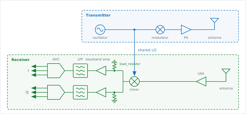
The transmit chain generates the waveform, modulates it, amplifies it and
radiates it. The receive chain amplifies the echo and mixes it against a
tap of the same source, so the baseband output carries the difference
between the transmitted and the received signal. The mixer feeds an I and a
Q branch — that pair is what bb_type="complex" returns, and a real
baseband keeps only one of them.#
Because the local oscillator is shared, the baseband signal is fully coherent with the transmit waveform. That single fact is what makes range appear as a beat frequency in an FMCW system, and what makes phase noise partially cancel for close-in targets — see Noise Simulation.
Two consequences are worth stating up front:
There is no separate IF stage to configure. The mixer output is the simulated baseband. Everything from the antenna to the ADC is described by
radarsimpy.Receiver.The deramp reference is a delayed copy of the transmit waveform. By default the delay is zero;
gate_delaymoves it, which is what makes long-range stretch processing possible (Long-Range Stretch Processing).
From Objects to Baseband#
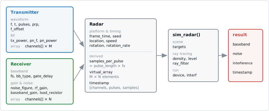
Transmitter and Receiver are pure configuration. Radar binds
them to a platform and derives the timing and array geometry. sim_radar
adds the scene and produces the output arrays.#
A minimal end-to-end configuration:
from radarsimpy import Radar, Transmitter, Receiver
from radarsimpy.simulator import sim_radar

wavelength = 3e8 / 79e9

tx = Transmitter(
    f=[77e9, 81e9],      # 4 GHz sweep
    t=[0, 40e-6],        # 40 us chirp
    tx_power=15,
    pulses=128,
    prp=50e-6,
    channels=[{"location": (0, 0, 0)}],
)

rx = Receiver(
    fs=20e6,
    noise_figure=8,
    rf_gain=20,
    baseband_gain=30,
    load_resistor=500,
    channels=[
        {"location": (0, i * wavelength / 2, 0)} for i in range(4)
    ],
)

radar = Radar(transmitter=tx, receiver=rx)

result = sim_radar(radar, targets=[{"location": (50, 0, 0), "rcs": 10}])
baseband = result["baseband"] + result["noise"]
The division of responsibility is strict:
Object |
Owns |
|---|---|
|
The waveform in time and frequency, how many pulses there are and how they are spaced, transmit power and phase noise, and the transmit array. See Transmitter and Waveform. |
|
Sampling rate and baseband type, the gain and noise budget from antenna to ADC, the range gate, and the receive array. See Receiver and Baseband. |
|
Where the platform is and how it moves, when frames start, and the
random seed. Everything else on |
|
The scene: targets, ray-tracing settings, interference and the execution device. See Ray-Tracing Simulation. |
What the Radar Derives#
Constructing a Radar computes three things that neither the transmitter nor
the receiver could know on its own.
Samples per pulse#
The receive window is open for one pulse length, so
This is the only place the transmitter’s timing and the receiver’s sampling
rate meet, and it is a hard constraint: the product must be at least 1, or the
constructor raises. Read it back with radar.samples_per_pulse.
Note
Choose fs and pulse_length so that the product is an exact integer.
Values that land a hair below an integer in binary — fs = N / 20e-6 for
power-of-two N is the classic case — are snapped to the nearest integer,
but keeping the product clean avoids the question entirely.
The virtual array#
With \(M\) transmit channels and \(N\) receive channels the simulator produces \(M \times N\) virtual elements, each at the vector sum of a transmit and a receive location:
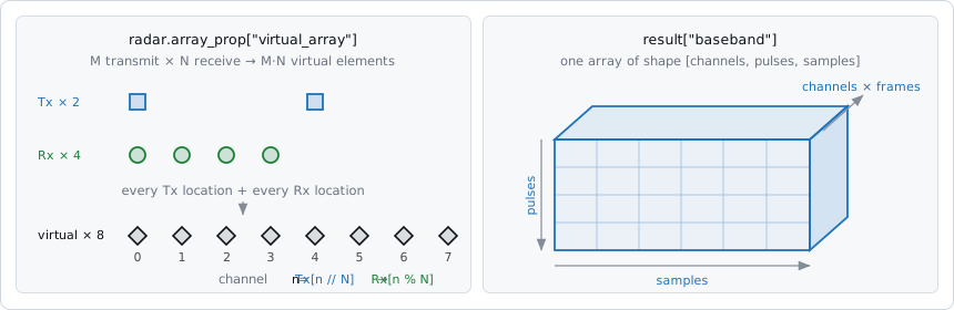
Left: two transmit elements spaced by the full receive aperture give eight
uniformly spaced virtual elements out of six physical ones. Right: the
returned arrays are indexed [channel, pulse, sample].#
The ordering is fixed, with the receive index varying fastest:
ch[0]       = Tx0 -> Rx0
ch[1]       = Tx0 -> Rx1
...
ch[N-1]     = Tx0 -> Rx(N-1)
ch[N]       = Tx1 -> Rx0
...
ch[M*N-1]   = Tx(M-1) -> Rx(N-1)
so channel n corresponds to Tx[n // N] and Rx[n % N]. The element
positions are available as radar.virtual_array_locations, an [M*N, 3]
array.
Note
The simulator returns these \(M \times N\) channels already separated, whatever the transmit channels happen to be doing at the time — see Simultaneous Transmit Channels. Real hardware has to earn that separation with TDM, CDM or DDM; Transmitter and Waveform covers the controls that do it.
The timestamp#
radar.time_prop["timestamp"] holds the absolute time of every sample,
shaped [channels, pulses, samples] like the baseband. It is assembled from
four contributions:
timestamp[ch, p, s] = frame_start_time            # Radar(frame_time=...)
                    + delay[ch // N]              # Tx channel delay
                    + pulse_start_time[p]         # cumsum(prp) - prp[0]
                    + gate_delay + s / fs         # receive window
This array is also the time base for time-varying motion. Target and radar
trajectories are written as functions of radar.time_prop["timestamp"] and
indexed positionally by the simulator, so anything that shifts the timestamps —
a transmit delay, a range gate, a non-uniform PRP — shifts the motion sampling
with them.
Noise amplitude#
The thermal-noise standard deviation follows from the receiver’s gain and
bandwidth budget alone. It is computed once at construction and stored in
radar.sample_prop["noise"]; the chain is laid out in Receiver and Baseband.
Frames#
frame_time repeats the whole configuration at a list of start times. The
per-frame blocks stack along the same first axis as the channels, with the
frame index varying slowest:
radar = Radar(transmitter=tx, receiver=rx, frame_time=[0, 0.1, 0.2])

result = sim_radar(radar, targets)
# result["baseband"].shape == (3 * M * N, pulses, samples)

cube = result["baseband"].reshape(3, M * N, pulses, samples)
Each frame gets an independent thermal-noise realization. Within a frame, all virtual channels that share a physical receiver and a timestamp get identical noise; Noise Simulation covers what that means for covariance estimation.
Simultaneous Transmit Channels#
sim_radar computes every transmit–receive path in isolation. Channel
n of the returned array holds only the energy that Tx[n // N] radiated
and Rx[n % N] collected, regardless of what the other transmitters were
doing at that instant. Adding a second transmitter does not disturb the first
one’s channel:
two = sim_radar(radar_2tx, targets)["baseband"]   # 2 Tx × 1 Rx → 2 channels
one = sim_radar(radar_1tx, targets)["baseband"]   # the same scene, Tx0 only

np.allclose(two[0], one[0])   # True — bit for bit
Real hardware does not behave that way. A physical receiver collects the sum of everything radiating while its window is open, and the whole job of a MIMO modulation scheme is to make that sum separable again after digitising. The simulator hands you the result of a perfect separation and skips the sum, so when you want the superposition you have to build it yourself.
Why it works this way#
There is no MIMO mode switch in the API. TDM, CDM, DDM and intra-pulse coding
are not options you select — they are what emerges from combining a per-channel
delay, a pulse_phs sequence, a mod_t / phs table and
f_offset (Transmitter and Waveform). That is the point of building the
transmitter out of primitives: it lets you model a scheme the library has never
heard of. But it also means the simulator has no way to infer which scheme you
had in mind. It cannot know which transmitters are meant to overlap, nor how
you intend to pull them apart again, so it does not guess.
The same choice is what puts unusual waveforms within reach. f and t
describe an arbitrary frequency-versus-time law instead of selecting from a
list, and mod_t / amp / phs carry an arbitrary complex envelope
through the pulse. Between them they describe a waveform rather than name
one: non-linear FM, stepped frequency, phase-coded PMCW, an OFDM symbol built
by loading subcarriers and taking an IFFT — and, on the same terms, schemes
that do not exist yet. The simulator never needs to have heard of a waveform
for it to be simulated; the waveform only has to be expressible as
\(f(t)\) and a complex envelope.
Note
One boundary is worth knowing about. The fast-time table is indexed by time within a pulse, so it repeats identically from pulse to pulse. A single symbol — one OFDM symbol, one phase code — is direct. A frame that carries different data in every symbol, as a full OFDM data frame or an OTFS grid does, is not expressible in a single call: build it from several and assemble the frame yourself. That this works at all is the same property again — nothing comes back pre-mixed.
The asymmetry settles the question. Superimposing channels is a one-line sum.
Recovering the individual paths from a sum is, in general, impossible — and no
more possible for the simulator than for you. So sim_radar returns the
finest decomposition it computed and leaves composition to the caller, where
the knowledge of the scheme actually lives.
The same rule shapes the rest of the return value. baseband holds the
target response with no thermal noise in it at all, while noise and
interference come back as separate arrays of the same shape. Nothing is
pre-mixed. You add the components you want and omit the ones you do not, which
is what makes it straightforward to compute a noise-free reference, isolate an
interference contribution, or take a single transmit–receive path on its own to
check a geometry.
Keeping the paths apart costs nothing, either. Every Tx–Rx pair already has its
own delay, Doppler, antenna-pattern weighting and polarization, so the engine
evaluates it separately whether or not the result is summed afterwards. And
because timestamp carries the same [channel, pulse, sample] layout, the
per-channel outputs stay aligned with per-channel time bases — which genuinely
differ the moment a transmitter is given a delay.
Building the physical receive signal#
Sum the transmit channels that share a receiver. The first axis runs frame, then Tx, then Rx, so a reshape does it:
import numpy as np

M = radar.transmitter.num_channels
N = radar.receiver.num_channels
P = radar.transmitter.num_pulses
S = radar.samples_per_pulse
K = np.size(radar.time_prop["frame_start_time"])

result = sim_radar(radar, targets)

signal = result["baseband"].reshape(K, M, N, P, S).sum(axis=1)
noise = result["noise"].reshape(K, M, N, P, S)[:, 0]

physical = signal + noise      # [frames, Rx, pulses, samples]
Important
Sum the signal, but take the noise once. Every virtual channel sharing a
physical receiver and a timestamp carries an identical noise realization,
so summing result["noise"] alongside the baseband multiplies the noise
amplitude by \(M\) — those are \(M\) copies of one draw, not
\(M\) independent ones. A real receiver has one front end and one noise
process, which is what the [:, 0] above keeps.
When it matters#
TDM — a per-channel delay puts each transmitter in its own time slot,
so the channels never overlap to begin with. The simulator’s per-path output
already matches what the hardware yields once the slots are de-interleaved.
Nothing to do.
CDM and DDM — the transmitters radiate together and are pulled apart afterwards, by code or by Doppler. Superimposing is what lets you see what the demodulator actually faces: residual cross-talk between codes, the way a target’s own Doppler mixes with a DDM phase ramp, and the dynamic range the ADC needs to hold \(M\) overlapping returns at once.
No modulation at all — several transmitters at different locations sending identical waveforms simultaneously are not separable by anything. The simulator still returns \(M \times N\) tidy channels; the hardware would return \(N\) channels of superimposed echoes with no way back to the individual paths. Building a virtual array from the simulator output here describes an array that could not be built.
Note
None of this forbids using the \(M \times N\) channels directly. Ideal separation is the right model for plenty of work — array geometry, angle estimation, beampattern studies — and it is both faster and cleaner than simulating a scheme only to undo it. The point is to choose deliberately rather than by default.
See Also#
Transmitter and Waveform — waveform, pulse train and transmit array
Receiver and Baseband — sampling, gain, noise budget and receive array
Coordinate Systems — how
locationandrotationare interpretedNoise Simulation — thermal noise and phase noise
Ray-Tracing Simulation — the scene side of
sim_radarRadar Model — full API reference for the three classes