Animated Targets (glTF 2.0 / GLB)#

A target’s motion is normally written by hand as speed and rotation_rate in its target dictionary. That works for a rigid body moving at a constant velocity and a constant rate, but many 3D assets already carry their motion inside the file: a drone with spinning rotors, a wind turbine, a car with turning wheels, or any object following a keyframed path.

radarsimpy.animation_kit reads that motion from a glTF 2.0 / GLB model and turns it into ordinary target dictionaries, so nothing else about your simulation changes.

Quick start#

import radarsimpy
from radarsimpy.animation_kit import load_animated_targets
from radarsimpy.simulator import sim_radar

radar = radarsimpy.Radar(transmitter=tx, receiver=rx)

targets = load_animated_targets(
    "turbine.glb",
    radar,
    location=(80, 0, 0),
    permittivity="PEC",
)

data = sim_radar(radar, targets)

load_animated_targets returns a plain list of target dictionaries. You can inspect them, edit them, or mix them with hand-written targets before passing them to radarsimpy.sim_radar().

Install the optional parser first:

pip install pygltflib

How the mapping works#

One target per animated node. Every glTF node that an animation channel targets becomes its own RadarSimPy target. Geometry beneath a node is grouped into the nearest animated ancestor, so each target moves as one rigid body. Meshes with no animated ancestor are merged into a single static target (merge_static=False keeps them separate).

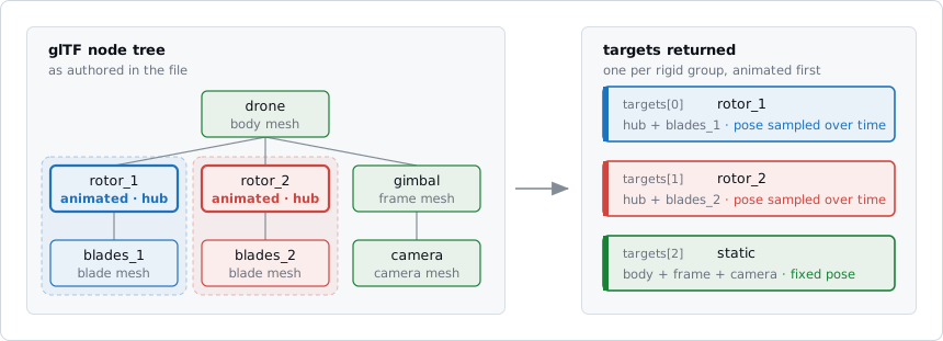
Each animated glTF node becomes one target holding its own mesh and every static mesh beneath it — A drone with two animated rotor nodes. Each rotor takes its own hub and the blades beneath it, because it is their nearest animated ancestor. The body, gimbal and camera have no animated ancestor, so they merge into one static target. Animated parts come first in the returned list.#

Motion is sampled at the radar’s own timestamps. The node’s world pose is evaluated at every entry of radar.time_prop["timestamp"] and emitted as time-varying location and rotation arrays, exactly the form the simulator already accepts for hand-written motion.

Velocity is analytic, not differenced. speed and rotation_rate are taken from the derivative of the keyframe interpolation itself. RadarSimCpp derives hit-point velocity from those two keys rather than from successive positions, so getting them right is what makes the Doppler correct.

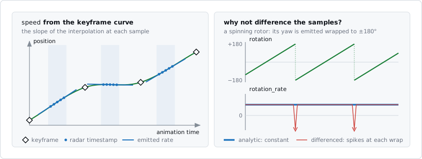
Rates are the slope of the keyframe interpolation at each radar timestamp; differencing the wrapped angles would spike — Left: radar timestamps arrive in short bursts, one per pulse. At each one, the emitted rate is the slope of the curve through the keyframes, whatever the gap to the next sample. Right: a spinning rotor’s `rotation` is emitted wrapped to ±180°. Differencing it would put a spurious −360°/Δt spike in `rotation_rate` at every wrap. The analytic rate stays constant.#

Frames are converted. glTF is Y-up; RadarSimPy is Z-up (see Coordinate Systems). Geometry, poses and rates are rotated accordingly. Pass up_axis="z" for an asset already exported Z-up.

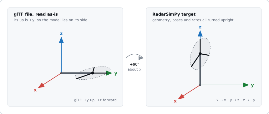
A Y-up glTF model read directly in the Z-up frame lies on its side; a +90 degree turn about x stands it upright — A wind turbine authored Y-up, drawn in RadarSimPy’s axes. Read as-is, its tower lies along +y. The default `up_axis="y"` applies a +90° turn about x, which stands the tower on +z and points the glTF +z forward axis along −y.#

Placing and driving the whole model#

The location, rotation, speed and rotation_rate arguments place and drive the complete model on top of its internal animation. A drone flying past while its rotors spin is:

targets = load_animated_targets(
    "drone.glb",
    radar,
    location=(60, -20, 15),
    speed=(0, 12, 0),
)

Controlling playback#

targets = load_animated_targets(
    "walk.glb", radar,
    animation="walk_cycle",  # name or index; default is the first clip
    time_offset=0.3,         # animation time at simulation time zero
    time_scale=1.5,          # play the clip 1.5x faster
    loop=True,               # wrap when the simulation outlasts the clip
)

With loop=False the first and last poses are held instead, and the rates go to zero outside the clip.

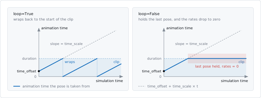
Simulation time maps to animation time through time_offset and time_scale; loop wraps past the end of the clip, otherwise the last pose is held — Simulation time `t` maps to animation time as `time_offset + time_scale × t` (dashed). With `loop=True` that value wraps back to the start of the clip each time it passes the end. With `loop=False` the last pose is held, and `speed` and `rotation_rate` are zero from then on.#

Static snapshots for RCS and lidar#

radarsimpy.sim_rcs() and radarsimpy.sim_lidar() do not accept time-varying motion. Ask for a single instant instead, which returns targets with ordinary scalar motion:

targets = load_animated_targets("turbine.glb", at_time=0.25)
rcs = sim_rcs(targets, f=77e9, inc_phi=0, inc_theta=90)

Inspecting the parts#

radarsimpy.animation_kit.load_animated_model() exposes the split without sampling anything, which is useful for checking how a model decomposes:

model = load_animated_model("drone.glb")
print(model["animations"], model["duration"])
for part in model["parts"]:
    print(part["name"], part["animated"], len(part["cells"]), "faces")

Animated targets also work with radarsimpy.mesh_kit.get_target_mesh() and radarsimpy.get_scene_state(), so you can plot the transformed geometry at any query time.

What is supported#

Feature	Status
`.gltf` and `.glb`	Supported
Node `translation` / `rotation` animation	Supported
`STEP`, `LINEAR` and `CUBICSPLINE` interpolation	Supported
Nested node hierarchies	Supported
Uniform, constant scale	Supported (baked into the geometry)
Skinning (`skins`, `JOINTS_0` / `WEIGHTS_0`)	Not supported
Morph targets (`weights` animation)	Not supported
Animated scale	Not supported
Non-uniform scale on an animated node	Not supported
Non-triangle primitives	Not supported

The unsupported cases all move individual vertices, while the ray tracer transforms each target rigidly. They raise a descriptive NotImplementedError rather than producing a silently wrong result. To simulate a deforming object such as a walking pedestrian, split it into rigid parts and animate their nodes instead.

Limitations to keep in mind#

Memory. Each animated part allocates twelve float32 arrays the size of radar.time_prop["timestamp"]. For a 4-channel, 256-pulse, 512-sample record that is roughly 25 MB per part, so a twenty-part model approaches 500 MB. This is inherent to the time-varying motion path, whose arrays must match the baseband time matrix. Merge parts that do not move independently to reduce it.

Gimbal lock. Poses are emitted as [yaw, pitch, roll]. At a pitch of ±90° the yaw and roll split becomes ambiguous, and a warning is issued. Avoid authoring motion that passes exactly through the pole.

Trial-version mesh limit. The face-count cap applies per target, and each animated part is its own target.