Receiver and Baseband

radarsimpy.Receiver describes the path from the receive antenna to the ADC: the array geometry and patterns, the gain and noise budget, where the receive window sits, and how the baseband is sampled.

Because the mixer deramps against the transmit oscillator (Radar System Model), the receiver has no independent frequency plan to configure — what it does have is a sampling rate, a gain chain, and a range gate.

The Signal Chain

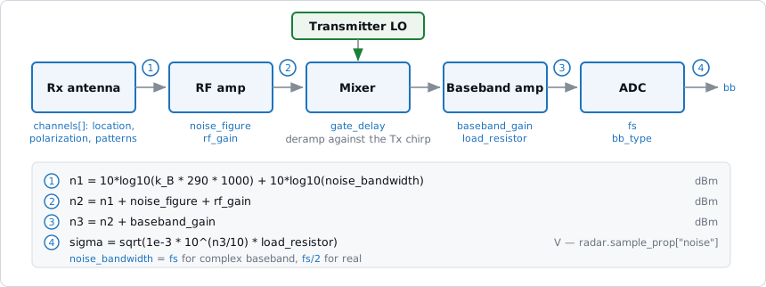
Each block carries the parameters that configure it. The ledger below tracks thermal noise from the antenna to the ADC; the result is the standard deviation of the noise added to every baseband sample.

Nothing in the chain is optional — a receiver constructed with only fs uses the defaults (noise_figure=10, rf_gain=0, baseband_gain=0, load_resistor=500), which still produce a well-defined noise level.

Sampling

fs is the baseband sampling rate, and it sets the number of samples taken during each pulse:

\[\text{samples\_per\_pulse} = \text{pulse\_length} \times f_s\]

The receive window is exactly one pulse_length long. It opens gate_delay after each pulse starts and closes pulse_length later; it does not extend into the idle time between pulses.

Note

Pick fs so that pulse_length * fs is an exact integer. The constructor snaps values that fall within rounding noise of an integer, but a clean product avoids any ambiguity between the Python and C++ sample counts.

Complex vs. real baseband

bb_type selects between a complex (I/Q) and a real baseband. The choice has three consequences:

	bb_type="complex" (default)	bb_type="real"
Output dtype	Complex	Real
noise_bandwidth	fs	fs / 2
Beat sign	Resolved — positive and negative beats are distinguishable	Not resolved — a target above the gate is indistinguishable from one the same distance below it

The noise bandwidth difference is why an otherwise identical real-baseband receiver reports a lower noise amplitude: it integrates over half the bandwidth, for \(\sqrt{2}\) less noise voltage.

Range span for deramped FMCW

For a linear FM waveform, range maps onto beat frequency through the chirp slope, so fs limits the recoverable range span:

\[\text{span} = \frac{B_\text{usable} \cdot c}{2 \left| k \right|}\]

where \(k\) is the chirp slope and \(B_\text{usable}\) is fs for complex baseband and fs/2 for real. Both are available on the radar:

>>> radar.chirp_slope
1e+14
>>> radar.unambiguous_range_span
29.98
>>> radar.unambiguous_range_window
(0.0, 29.98)

A 4 GHz sweep in 40 µs is a slope of 100 MHz/µs, so 20 MHz of complex baseband covers only 30 m. Widening that span means a faster ADC, a slower sweep, or a range gate.

Note

These properties describe deramp (stretch) processing of a linear FM waveform. They return None for CW, pulsed and arbitrary waveforms, where range does not map onto beat frequency.

The Noise Budget

The thermal-noise standard deviation is computed once, when the Radar is constructed, and stored in radar.sample_prop["noise"]. It follows the ledger in the figure above:

n1    = 10*log10(k_B * 290 * 1000) + 10*log10(noise_bandwidth)   [dBm]
n2    = n1 + noise_figure + rf_gain                              [dBm]
n3    = n2 + baseband_gain                                       [dBm]
sigma = sqrt(1e-3 * 10**(n3/10) * load_resistor)                 [V]

The reference temperature is fixed at 290 K. Worked through for a typical front end:

Step	Expression	Value
Thermal floor, fs = 20 MHz complex	\(-174 + 73.0\)	−101.0 dBm
After the RF amp, noise_figure=8, rf_gain=20	\(-101.0 + 28\)	−73.0 dBm
After the baseband amp, baseband_gain=30	\(-73.0 + 30\)	−43.0 dBm
In volts across load_resistor=500	\(\sqrt{10^{-3} \cdot 10^{-4.3} \cdot 500}\)	5.03 mV

from radarsimpy import Radar, Transmitter, Receiver

tx = Transmitter(f=[77e9, 81e9], t=[0, 40e-6], pulses=128, prp=50e-6)
rx = Receiver(
    fs=20e6,
    noise_figure=8,
    rf_gain=20,
    baseband_gain=30,
    load_resistor=500,
)
radar = Radar(transmitter=tx, receiver=rx)

radar.sample_prop["noise"]   # 0.005026...

Two things about this that regularly surprise people:

• The gains are not free. rf_gain and baseband_gain amplify the signal and the noise equally, so raising them changes the absolute scale of the baseband but not the SNR. Only noise_figure and noise_bandwidth move the SNR.

• The noise is not added for you. sim_radar returns the clean response in result["baseband"] and the noise realization separately in result["noise"]; add them to get a noisy measurement.

Noise Simulation covers the statistics of the generated noise, its correlation structure across MIMO virtual channels, and the transmitter phase-noise model.

The Range Gate

gate_delay moves the receive window and the deramp reference together, by the same amount. A target at range c * gate_delay / 2 then produces a DC beat, and targets around it beat at 2 * k * dR / c:

gate_range = 111.12e3                        # m
rx = Receiver(fs=40e6, gate_delay=2 * gate_range / 299792458)

rx.gate_range     # 111120.0

With the default of 0 the reference sits at zero delay, which is fine at short range and impossible at long range: the beat frequency k * tau grows without bound with the round-trip delay and passes Nyquist long before real long-range radars operate. Long-Range Stretch Processing works through the arithmetic and the caveats — including how gate_delay interacts with per-pulse f_offset and phase codes.

Receive Channels

channels is a list of dictionaries, one per receive element, and location is the only required key.

Key	Default	Meaning
location	—	[x, y, z] in metres, relative to the radar origin.
polarization	[0, 0, 1]	Antenna polarization vector. Vertical [0, 0, 1], horizontal [0, 1, 0], right-hand circular [0, 1, 1j], left-hand circular [0, 1, -1j].
azimuth_angle / azimuth_pattern	[-90, 90] / [0, 0]	Matched arrays of angle (degrees) and gain (dB).
elevation_angle / elevation_pattern	[-90, 90] / [0, 0]	Same, in elevation.

The pattern convention matches the transmitter: the peak of the azimuth pattern becomes the channel’s antenna gain and the azimuth pattern is normalized to it, while the elevation pattern is normalized to its own peak and contributes shape only. Put absolute gain in the azimuth cut.

A half-wavelength uniform linear array along the y axis:

import numpy as np
from radarsimpy import Receiver

wavelength = 3e8 / 79e9
rx = Receiver(
    fs=20e6,
    noise_figure=8,
    rf_gain=20,
    baseband_gain=30,
    channels=[
        {"location": (0, i * wavelength / 2, 0)} for i in range(8)
    ],
)

Receive locations combine with transmit locations to form the virtual array; the ordering is described in Radar System Model.

Reading the Configuration Back

rx.sampling_rate        # fs
rx.noise_bandwidth      # fs or fs/2, per bb_type
rx.gate_delay           # s
rx.gate_range           # gate_delay * c / 2, m
rx.num_channels
rx.channel_locations    # [N, 3]
rx.get_channel_info(0)  # location, polarization, gain, patterns

See Also

• Radar System Model — how the receiver combines with the transmitter

• Transmitter and Waveform — the other half of the transceiver

• Noise Simulation — noise statistics and MIMO correlation structure

• Long-Range Stretch Processing — range gating for long-range FMCW

• Doppler Sign Convention — the sign of the Doppler frequency in the baseband

• Coordinate Systems — angle and orientation conventions

• Radar Model — full Receiver API reference